Introduction
Welcome to the tutorials! Here we will learn how to make a computational research project reproducible using several different tools, described in the figure below:
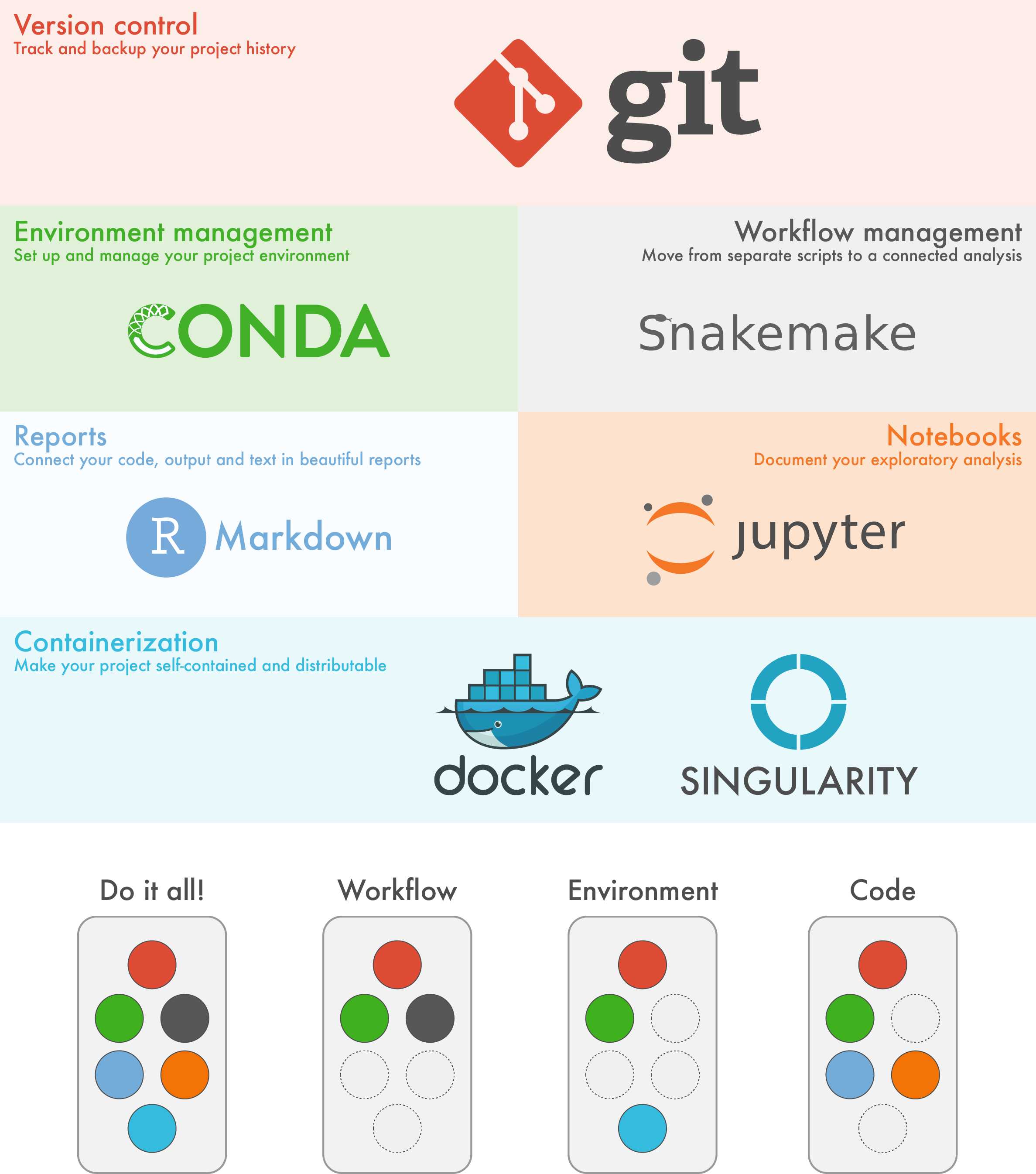
The figure gives an overview of the six available tutorials, a very brief description of their main purpose, and the suggested order to do them. However, each tutorial is made so that it can be completed independently of the other tutorials. It is therefore perfectly possible to choose a different order, or a subset of tutorials that suits your interests. Under the main figure there is a list of a few suggested alternative tutorial orders; you will find the tutorials in the menu to the left.
Before going into the tutorials themselves, we first describe the case study from which the example data comes from, followed by the setup needed to install the tools themselves. These will create quite a lot of files on your computer, some of which will actually take up a bit of storage space too. In order to remove any traces of these after completing the tutorials, please refer to the Take down section.
The case study
We will be running a small bioinformatics project as a case study, and use that to exemplify the different steps of setting up a reproducible research project. To give you some context, the study background and analysis steps are briefly described below.
Background
The data is taken from Osmundson, Dewell, and Darst (2013), who have studied methicillin-resistant Staphylococcus aureus (MRSA). MRSA is resistant to broad spectrum beta-lactam antibiotics and lead to difficult-to-treat infections in humans. Lytic bacteriophages have been suggested as potential therapeutic agents, or as the source of novel antibiotic proteins or peptides. One such protein, gp67, was identified as a transcription-inhibiting transcription factor with an antimicrobial effect. To identify S. aureus genes repressed by gp67, the authors expressed gp67 in S. aureus cells. RNA-seq was then performed on three S. aureus strains:
- RN4220 with pRMC2 with gp67
- RN4220 with empty pRMC2
- NCTC8325-4
Analysis
The graph below shows the different steps of the analysis that are included in this project:

The input files are:
- RNA-seq raw data (FASTQ files) for the three strains
- S. aureus genome sequence (a FASTA file)
- S. aureus genome annotation (a GFF file)
The different steps of the workflow and what they do are as follows:
get_genome_fasta- Download the genome file.index_genome- Index the genome using the Bowtie2 software (required for the alignment step)get_SRA_by_accession- Download the RNA-seq raw data for the three strains from the Sequence Read Archive (SRA).fastqc- Run quality control on each of the RNA-seq FASTQ files using the FastQC software.multiqc- Summarize the quality controls.align_to_genome- Align the RNA-seq data from the three strains to the indexed genome using the Bowtie2 software.sort_bam- Sort the alignment files by genome coordinate using the Samtools software.get_genome_gff3- Download the genome annotation file.generate_count_table- Calculate gene expression by counting aligned reads per gene using the HTSeq-count software.generate_rulegraph- Generate the workflow overview figure shown above.make_supplementary- Produce the supplementary materials section using data from the quality controls, gene counts and the workflow figure.