Introduction to R Markdown
Markup
A markup language is a system for annotating text documents in order to e.g. define formatting. HTML, if you are familiar with that, is an example of a markup language. HTML uses tags, such as:
<h1>Heading</h1>
<h2>Sub-heading</h2>
<a href="www.webpage.com">Link</a>
<ul>
  <li>List-item1</li>
  <li>List-item2</li>
  <li>List-item3</li>
</ul>
Markdown is a lightweight markup language which uses plain-text syntax in order to be as unobtrusive as possible, so that a human can easily read it. Some examples:
# Heading

## Sub-heading

### Another deeper heading

A [link](http://example.com).

Text attributes _italic_, *italic*, **bold**, `monospace`.

Bullet list:

  * apples
  * oranges
  * pears
A markdown document can be converted to other formats, such as HTML or PDF, for viewing in a browser or a PDF reader (the page you are reading right now is written in markdown). Markdown is somewhat ill-defined, and as a consequence of that there exists many implementations and extensions (although they share most of the syntax). R Markdown is one such implementation/extension.
R Markdown
R Markdown documents can be used both to save and execute code (with a focus on R) and to generate reports in various formats. This is done by mixing markdown (as in the example above), and so-called code chunks in the same document. The code itself, as well as the output it generates, can be included in the final report.
R Markdown makes your analysis more reproducible by connecting your code, figures and descriptive text. You can use it to make reproducible reports, rather than e.g. copy-pasting figures into a Word document. You can also use it as a notebook, in the same way as lab notebooks are used in a wet lab setting (or as we us a Jupyter notebook in the tutorial).
The best way to understand R Markdown is by using it, so head down to the practical exercise below to learn more!
Tell me more
- A nice "Get Started" section, as a complement to this tutorial, is available at RStudio.com.
- R Markdown cheat sheet (also available from Help > Cheatsheets in RStudio)
- R Markdown reference guide (also available from Help > Cheatsheets in RStudio)
Set up
This tutorial depends on files from the course Bitbucket repo. Take a look at the intro for instructions on how to set it up if you haven't done so already. Then open up RStudio and set your working directory to reproducible_research_course/rmarkdown.
Install RStudio and R
If you don't already have R or RStudio, you will need to install them:
- Download and install R following the instructions here.
- Download and install RStudio Desktop (free) following the instructions here.
Windows users
Although most of the tutorials are best to run in a Docker container or in the Linux Bash Shell if you are a Windows user (see information in the intro), both R and RStudio run well directly on Windows. It is therefore suggested that you install Windows versions of these software (if you haven't done so already) when doing this tutorial.
Practical exercise
Getting started with R Markdown
- Start RStudio
- Select: File > New File > R Markdown
- You might get prompted to install a few required packages. Do that in such case!
- In the window that opens, select: Document and HTML (should be default), and click Ok.
- This will open a template R Markdown document for you
On the top is a so called YAML header:
---
title: "Untitled"
output:
  html_document:
    toc: true
---
Attention
The header might look slightly different depending on your version of RStudio. If so, replace the default with the header above.
Here we can specify settings for the document, like the title and the output format.
- Change the title to "My first R Markdown document".
- Now, read through the rest of the template R Markdown document to get a feeling for the format.
As you can see, there are essentially three types of components in an R Markdown document:
- Text (written in R Markdown)
- Code chunks (written in R, or another supported language).
- The YAML header
Let's dig deeper into each of these in the following sections! But first, just to get a flavor for things: press the little Knit-button located at the top of the text editor panel in RStudio. This will prompt you to save the Rmd file (do that), and generate the output file (an HTML file in this case). It will also open up a preview of this file for you.
Markdown text
Some commonly used formatting written in markdown is shown below:
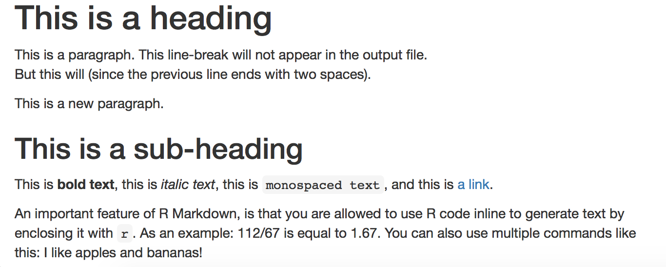
# This is a heading

This is a paragraph.
This line-break will not appear in the output file.
But this will (since the previous line ends with two spaces).

This is a new paragraph.

## This is a sub-heading

This is **bold text**, this is *italic text*, this is `monospaced text`,
and this is [a link](http://rmarkdown.rstudio.com/lesson-1.html).

An important feature of R Markdown, is that you are allowed to use R code inline
to generate text by enclosing it with `r `.
As an example: 112/67 is equal to `r round(112/67, 2)`.
You can also use multiple commands like this:
I like `r fruits <- c("apples","bananas"); paste(fruits, collapse=" and ")`!
The above markdown would generate something like this:
Instead of reiterating information here, take a look on the first page (only the first page!) of this reference. This will show you how to write more stuff in markdown and how it will be displayed once the markdown document is converted to an output file (e.g. HTML or PDF). An even more complete guide is available here.
- Try out some of the markdown described above (and in the links) in your template R Markdown document! Press Knit to see the effect of your edits. Don't worry about the code chunks just yet, we'll come to that in a second.
Quick recap
In this section you learned and tried out some of the basic markdown syntax.
Code chunks
Enough about markdown, let's get to the fun part and include some code! Look at the last code chunk in the template R Markdown document that you just created, as an example:
```{r pressure, echo = FALSE}
plot(pressure)
```
The R code is surrounded by: ```{r} and ```. The r indicates that the code chunk contains R code (it is possible to add code chunks using other languages, e.g. Python). After that comes an optional chunk name, pressure in this case (this can be used to reference the code chunk as well as alleviate debugging). Last comes chunk options, separated by commas (in this case there is only one option: echo = FALSE).
Note
Note that the code chunk name pressure has nothing to do with the code plot(pressure). In the latter case, pressure is a default R dataframe that is used in examples. The chunk name happened to be set to the string pressure as well, but could just as well have been called something else, e.g. plot_pressure_data.
Below are listed some useful chunk options related to evaluating and displaying code chunks in the final file:
| Chunk option | Effect |
|---|---|
echo = FALSE |
Prevents code, but not the results, from appearing in the finished file. This is a useful way to embed figures. |
include = FALSE |
Prevents both code and results from appearing in the finished file. R Markdown still runs the code in the chunk, and the results can be used by other chunks. |
eval = FALSE |
The code in the code chunk will not be run (but the code can be displayed in the finished file). Since the code is not evaluated, no results can be shown. |
results = "hide" |
Evaluate (and display) the code, but don't show the results. |
message = FALSE |
Prevents messages that are generated by code from appearing in the finished file. |
warning = FALSE |
Prevents warnings that are generated by code from appearing in the finished file. |
- Go back to your template R Markdown document in RStudio and locate the
carscode chunk. - Add the option
echo = FALSE:
```{r cars, echo = FALSE}
summary(cars)
```
- Guess how this will affect the final file. Press Knit and look at the generated file. Were you right?
- Remove the
echo = FALSEoption and addeval = FALSEinstead:
```{r cars, eval = FALSE}
summary(cars)
```
- Guess how this will affect the final file. Press Knit and look at the generated file. Were you right?
- Remove the
eval = FALSEoption and addinclude = FALSEinstead:
```{r cars, include = FALSE}
summary(cars)
```
There are also some chunk options related to plots:
| Chunk option | Effect |
|---|---|
fig.height = 9, fig.width = 6 |
Set plot dimensions to 9x6 inches. (The default is 7x7.) |
out.height = "10cm", out.width = "8cm" |
Scale plot to 10x8 cm in the final output file. |
fig.cap = "This is a plot." |
Adds a figure caption. |
- Go back to your template R Markdown document in RStudio and locate the
pressurecode chunk. - Add the
fig.widthandfig.heightoptions as below:
```{r pressure, echo = FALSE, fig.width = 6, fig.height = 4}
plot(pressure)
```
- Press Knit and look at the output. Can you notice any difference?
- Now add a whole new code chunk to the end of the document. Give it the name
pressure2(code chunks have to have unique names, or no name). Add thefig.widthandout.widthoptions like this:
```{r pressure2, echo = FALSE, fig.width = 9, out.width = "560px"}
plot(pressure)
```
- Press Knit and look at the output. Notice the difference between the two plots? In the second chunk we have first plotted a figure that is a fair bit larger (9 inches wide) than that in the first chunk. Next we have down-sized it in the final output, using the
out.widthoption. (Here we need to use a size metric recognized by the output format, in this case "560px" which works for HTML.)
Have you noticed the first chunk?
```{r setup, include = FALSE}
knitr::opts_chunk$set(echo = TRUE)
```
In this way we can set global chunk options, i.e. defaults for all chunks. In this example, echo will always be set to TRUE, unless otherwise specified in individual chunks.
Tip
For more chunk options, have a look at page 2-3 of this reference.
It is also possible to create different types of interactive plots using R Markdown. You can see some examples of this
here. If you want to try it out, you can install e.g. the package networkD3 with install.packages("networkD3"). Then add the following code chunk to your document:
```{r}
library(networkD3)
data(MisLinks, MisNodes)
forceNetwork(Links = MisLinks, Nodes = MisNodes, Source = "source",
             Target = "target", Value = "value", NodeID = "name",
             Group = "group", opacity = 0.4)
```
Quick recap
In this section you learned how to include code chunks and how to use chunk options to control how the output (code, results and figures) is displayed.
YAML header
Last but not least, we have the YAML header. Here is where you configure general settings for the final output file, and a few other things.
The settings are written in YAML format in the form key: value. Nested settings or sub-settings are indented with spaces. In the template R Markdown document you can see that html_document is nested under output, and in turn, toc is nested under html_document since it is a setting for the HTML output. The table of contents (TOC) is automatically compiled from the section headers (marked by #).
- Add a subsection header somewhere in your document using three
###. Knit and look at how the table of contents is structured. - Now set
toc: falseand knit again. What happened? - A setting that works for HTML output is
toc_float: true. Add that to your document (same indentation level astoc: true) and knit. What happened? - In the same way, add the option
number_sections: true. What happened? - Think it looks weird with sections numbered with 0, e.g. 0.1? That is because the document does not contain any level-1-header. Add a header using only one
#at the top of the document, just after thesetupchunk. Knit and see what happens!
We can also set parameters in the YAML header. These are either character strings, numerical values, or logicals, and they can be used in the R code in the code chunks. Let's try it out:
- Add two parameters,
dataandcolor, to the YAML header. It should now look something like this:
---
title: "Untitled"
output:
  html_document:
    toc: true
    toc_float: true
    number_sections: true
params:
  data: cars
  color: blue
---
- So now we have two parameters that we can use in the code! Modify the
pressurecode chunk so that it looks like this:
```{r pressure, fig.width = 6, fig.height = 4}
plot(get(params$data), col = params$color)
```
This will plot the dataset cars using the color blue.
- Knit and see what happens!
Later, we will learn how to set parameters using an external command.
We have up until now mainly been using html_document as an output format. There are however a range of different available formats to choose between. What is important to know, is that not all chunk settings work for all output formats (this mainly regards settings related to rendering plots and figures), and some YAML settings are specific for the given output format chosen.
- Take a look at this gallery of R Markdown documents to see what different kinds of output formats are possible to generate.
- Take a look at the last page of this reference for a list of YAML header options, and what output formats they are available for.
Quick recap
In this section you learned how to set document-wide settings in the YAML header, including document output type and user defined parameters.
Managing and working with R Markdown documents
Below are a few practical things regarding working with R Markdown documents:
More about rendering
- You can knit/render reports in several different ways:
- By pressing the Knit button in RStudio (as we have done this far)
- By running the R command
render, e.g. to Knit the filemy_file.Rmdrunrender("my_file.Rmd")in the R console. - By running on the terminal command line:
R -e 'rmarkdown::render("my_file.Rmd")'
- Using the
rendercommand, we can also set YAML header options and change defaults (i.e. override those specified in the R Markdown document itself). Here are a few useful arguments (see?rmarkdown::renderfor a full list):output_format- change output format, e.g.html_documentorpdf_document.output_fileandoutput_dir- change directory and file name of the generated report file (defaults to the same name and directory as the .Rmd file).params- change parameter defaults. Note that only parameters already listed in the YAML header can be set, no new parameters can be defined.
Try to use the render command to knit your template R Markdown document and set the two parameters data and color. Hint: the params argument should be a list, so e.g.:
rmarkdown::render("my_file.Rmd", params=list(data="cars", color="green"))
Tips for working with R Markdown documents in RStudio
- You might already have noticed that you can run code chunks directly in RStudio:
- Place the cursor on an R command and press
CTRL + Enter(Windows) orCmd + Enter(Mac) to run that line in R. - Select several R command lines and use the same keyboard shortcut as above to run those lines.
- To the right in each chunk there are two buttons; one for running the code in all chunks above the current chunk and one for running the code in the current chunk (depending on your layout, otherwise you can find the options in the Run drop-down).
- Depending on your settings, the output of the chunk code will be displayed inline in the Rmd document, or in RStudios Console and Plot panels. To customize this setting, press the cog-wheel next to the Knit button and select either "Chunk Output Inline" or "Chunk Output in Console".
- Place the cursor on an R command and press
- You can easily insert an empty chunk in your Rmd document in RStudio by pressing Insert > R.
- In the top right in the editor panel in RStudio there is a button to toggle the document outline. By making that visible you can click and jump between sections (headers and named code chunks) in your R Markdown document.
Using R Markdown in the MRSA project
As you might remember from the intro, we are attempting to understand how lytic bacteriophages can be used as a future therapy for the multiresistant bacteria MRSA (methicillin-resistant Staphylococcus aureus). In this exercise we will use R Markdown to make a report in form of a Supplementary Material PDF based on the outputs from the Snakemake tutorial. Among the benefits of having the supplementary material (or even the full manuscript!) in R Markdown format are:
- It is fully transparent how the text, tables and figures were produced.
- If you get reviewer comments, or realize you've made a mistake somewhere, you can easily update your code and regenerate the document with the push of a button.
- By making report generation part of your workflow early on in a project, much of the eventual manuscript "writes itself". You no longer first have to finish the research part and then start creating the tables and figures for the paper.
Before you start:
- Make sure that your working directory in R is
rmarkdownin the course directory (Session > Set Working Directory). - Open the file
rmarkdown/code/supplementary_material.Rmd. - To complete this part you first need to install the following R-packages:
BiocManager::install("ggplot2")
BiocManager::install("reshape2")
BiocManager::install("pheatmap")
BiocManager::install("rtracklayer")
BiocManager::install("GEOquery")
Note
In this tutorial, for the sake of trying out R Markdown, we have installed R
and RStudio separately and now we install
individual R packages using the standard R procedure (using
install.packages() or BiocManager::install()). Nevertheless, it is
possible to install R, R packages and even RStudio through conda. If you
want to, you can try to install the above packages using conda instead
(we will do that later in the Docker tutorial). As conda packages, the
R packages above are called r-ggplot2, r-reshape2, r-pheatmap,
bioconductor-rtracklayer, and bioconductor-geoquery.
However, to get access to
the installed R packages in RStudio you will need to open RStudio from
the command line in the activated conda environment. On Mac you can do this
by open -a RStudio -n. In R, check the available library path by
.libPaths() to make sure that it points to a path within your conda environment.
It might be that .libPaths() shows multiple library paths, in which case
R packages will be searched for by R in both these locations. This means that
your R session will not be completely isolated in your conda environment, and
that something that works for you might not work for someone else usgin the same
conda environment, simply because you had additional packages installed in the
second library location. One way to force R to just use the conda library path
is to add a .Renviron file to the directory where you start R with these lines:
R_LIBS_USER=""
R_LIBS=""
.libPaths() now
only point to your conda environment, you will probably also need to install
r-rmarkdown.
- Let's start by taking a look at the YAML header at the top of the file. The parameters correspond to files (and sample IDs) that are generated by the MRSA analysis workflow (see the Snakemake tutorial) and contain results that we want to include in the supplementary material document. We've also specified that we want to render to PDF.
---
title: "Supplementary Material"
output: pdf_document
params:
  counts_file: "results/tables/counts.tsv"
  multiqc_file: "intermediate/multiqc_general_stats.txt"
  rulegraph_file: "results/rulegraph.png"
  SRR_IDs: "SRR935090 SRR935091 SRR935092"
  GSM_IDs: "GSM1186459 GSM1186460 GSM1186461"
---
- From a reproducibility perspective it definitely makes sense to include information about who authored the document and the date it was generated. Add the two lines below to the YAML header. Note that we can include inline R code by using
`r some_code`.
author: John Doe, Joan Dough, Jan Doh, Dyon Do
date: "`r format(Sys.time(), '%d %B, %Y')`"
Tip
Make it a practice to keep track of all input files and add them as parameters rather than hard-coding them later in the R code.
- Next, take a look at the
dependencies,read_params, andread_datachunks. They 1) load the required packages, 2) reads the parameters and stores them in R objects to be used later in the code, and 3) reads the data in the counts file, the multiqc file, as well as fetches meta data from GEO. These chunks are provided as is, and you do not need to edit them. - Below these chunks there is some markdown text that contains the Supplementary Methods section. Note the use of section headers using
#and##. - Then there is a Supplementary Tables and Figures section. This contains four code chunks, each for a specific table or figure. Have a quick look at the code and see if you can figure out what it does. Don't worry if you can't understand everything.
- Finally, there is a Reproducibility section which describes how the results in the report can be reproduced. The
session_infochunk prints information regarding R version and which packages and versions that are used. We highly encourage you to include this chunk in all your R Markdown reports. It's an effortless way to increase reproducibility. - Now that you have had a look at the R Markdown document, it is time to Knit! We will do this from the R terminal (rather than pressing Knit).
rmarkdown::render("code/supplementary_material.Rmd",
                  output_dir = "results")
The reason for this is that we can then redirect the output PDF file to be saved in the results/ directory.
Normally, while rendering, R code in the Rmd file will be executed using the directory of the Rmd file as working directory (rmarkdown/code in this case).
However, it is good practice to write all code as if it would be executed from the project root directory (rmarkdown/ in this case). For instance, you can see that we have specified the files in params with relative paths from the project root directory. To set a different directory as working directory for all chunks one modifies the knit options like this:
knitr::opts_knit$set(root.dir = normalizePath('../'))
Here we set the working directory to the parent directory of the Rmd file (../), in other words, the project root. Use this rather than setwd() while working with Rmd files.
- Take a look at the output. You should find the PDF file in the
resultsdirectory.
You will probably get a good idea of the contents of the file, but the tables look weird and the figures could be better formatted. Let's start by adjusting the figures!
- Locate the
setupchunk. Here, we have already setecho = FALSE. Let's add some default figure options:fig.height = 6, fig.width = 6, fig.align = 'center'.
This will make the figures slightly smaller than default and center them.
- Knit again, using the same R command as above. Do you notice any difference? Better, but still not perfect!
Let's improve the tables! We have not talked about tables before. There are several options to print tables, here we will use the kable function which is part of the knitr package.
- Go to the
sample-infochunk. Replace the last line,d, with:
knitr::kable(d)
- Knit again and look at the result. You should see a formatted table.
- The column names can be improved, and we could use a table legend. Change to use the following:
knitr::kable(d, caption="Sample info",
      col.names=c("SRR", "GEO", "Strain", "Treatment"))
- Knit and check the result.
- Try to fix the table in the
qc-statschunk in the same manner. The colnames are fine here, so no need to bother changing them, but add a table legend: "QC stats from FastQC". Knit and check your results.
Let's move on to the figures!
- Go to the
counts-barplotchunk. To add a figure legend we have to use a chunk option (so not in the same way as for tables). Add the chunk option:
fig.cap = "Counting statistics per sample, in terms of read counts for genes and reads not counted for various reasons."
- Knit and check the outcome!
- Next, add a figure legend to the figure in the
gene-heatmapchunk. Here we can try out the possibility to add R code to generate the legend:
fig.cap = paste("Expression (log-10 counts) of genes with at least ", max_cutoff, " counts in one sample and a CV>", cv_cutoff, ".", sep = "")
This will use the cv_cutoff and max_cutoff variables to ensure that the figure legend gives the same information as was used to generate the plot. Note that figure legends are generated after the corresponding code chunk is evaluated. This means we can use objects defined in the code chunk in the legend.
- Knit and have a look at the results.
You may have noticed that the figures (probably) aren't positioned relative to the text exactly where you put the code chunks? This is a feature of the LaTeX rendering to PDF, where it tries to align tables and figures in an aestetically pleasing and efficient way. These are called "floats" in LaTeX, and can be a source of frustration. If you want to force the floats to be positioned in the order and context they appear in the text, you can use the following tweak. Note that this is only an issue with rendering to PDF, not with e.g. HTML.
- Add the option
fig.pos = 'H'toopts_chunkin thesetupchunk (note the capital "H"). This will force figures to appear "here". Add the following lines to the header:
header-includes:
  \usepackage{float}
- Knit and admire the results!
The heatmap still looks a bit odd. Let's play with the fig.height and out.height options, like we did above, to scale the figure in a more appropriate way. Add this to the chunk options: fig.height=10, out.height="22cm". Knit and check the results. Does it look better now?
- Now let's add a third figure! This time we will not plot a figure in R, but use an available image file showing the structure of the Snakemake workflow used to generate the inputs for this report. Add a new chunk at the end of the Supplementary Tables and Figures section containing this code:
knitr::include_graphics(normalizePath(rulegraph_file))
- Also, add the chunk options:
fig.cap = "A rule graph showing the different steps of the bioinformatic analysis that is included in the Snakemake workflow."
and:
out.height = "11cm"
- Knit and check the results.
As previously mentioned, the rendering process to PDF will make use of LaTeX. In the last part we will see how we can add LaTeX commands directly in the R Markdown document to further customize the look.
- See the section on Reproducibility in the PDF. Notice that the R code output giving information about the R session is a bit big? We can fix this by adding the LaTeX commands
\footnotesizeand\normalsizebefore and after this part, i.e.:
\footnotesize
```{r session_info}
sessionInfo()
```
\normalsize
This will make the sessionInfo() text smaller and then set it back to normal.
- Knit and check the outcome.
- You may also notice that the heading "Reproducibility" would be better to place on a new page. To achieve this, insert
\newpagebefore the heading (make sure to have a blank line before and after\newpage). Knit and see if it worked. - The last things that we will fix are the figure and table labels. Now they are automatically called e.g. Figure 1 and Table 1, but perhaps we would like to name them Figure S1 and Table S1, being Supplementary. We can customize this using the separate LaTeX file,
code/header.tex. To include this in the Rmd, update the YAML header so that it looks like this. Note that we have now included\usepackage{float}in thecode/header.texfile insted of having it in the header. Keeping all your configuration settings in one file is a good way of achieving a consistant look for your report.
---
title: "Supplementary Material"
author: John Doe, Joan Dough, Jan Doh, Dyon Do
date: "`r format(Sys.time(), '%d %B, %Y')`"
output:
  pdf_document:
    includes:
      in_header: header.tex
params:
  counts_file: "results/tables/counts.tsv"
  multiqc_file: "intermediate/multiqc_general_stats.txt"
  rulegraph_file: "results/rulegraph.png"
  SRR_IDs: "SRR935090 SRR935091 SRR935092"
  GSM_IDs: "GSM1186459 GSM1186460 GSM1186461"
---
- Knit and view the results.
Quick recap
In this section you learned some additional details for making nice R Markdown reports in a reproducible research project setting, including setting the root directory, adding tables, setting figure and table captions, and using LaTeX commands for formatting details.
R Markdown and Snakemake
It is definitely possible to render R Markdown documents as part of a Snakemake workflow. This
is something we do for the final version of the MRSA project (in the Docker tutorial). In such
cases it is advisable to manage the installation of R and required R packages through your
conda environment file and use the rmarkdown::render() command from the shell section of your
Snakemake rule (see the Snakefile in docker/ for an example).
Using R Markdown for making slides
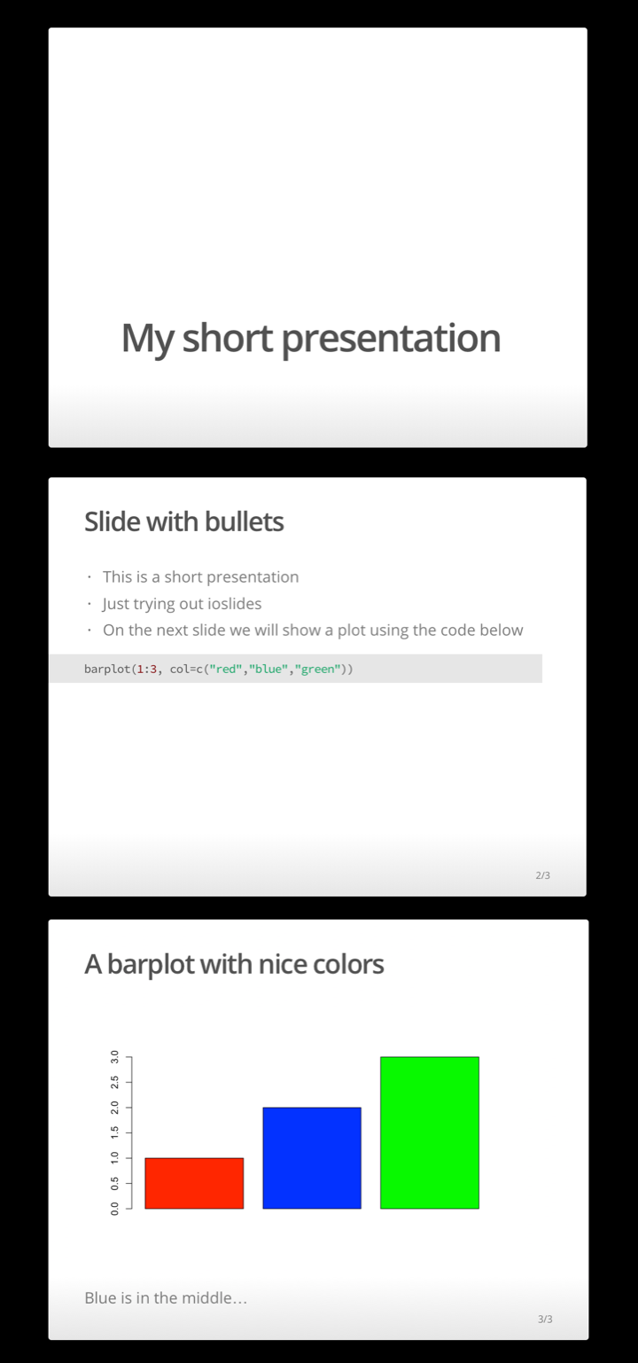
Lastly, if you have time, you can try out using R Markdown for making presentations.
The exercise task is short and simple: recreate the slides shown below using R Markdown (hint: use output format "ioslides").
Tip
It is now also possible to render PowerPoint presentations, but note that this requires rmarkdown >= v1.9 and Pandoc >= v2.0.5.
Congrats! You made it to the end and are now an R Markdown expert!