Introduction to Jupyter notebooks
The Jupyter Notebook is an open-source web application that allows you to create and share documents that contain code, equations, visualizations and text. The functionality is partly overlapping with R Markdown (see the tutorial), in that they both use markdown and code chunks to generate reports that integrate results of computations with the code that generated them. Jupyter Notebook comes from the Python community while R Markdown was developed by RStudio, but you could use most common programming languages in either alternative. In practice though, it's quite common that R developers use Jupyter but probably not very common that Python developers use RStudio.
What are Jupyter notebooks for?
An excellent question if I may say so! Some applications could be:
- Python is lacking a really good IDE for doing exploratory scientific data analysis, like RStudio or Matlab. Some people use it simply as an alternative for that.
- The community around Jupyter notebooks is large and dynamic, and there are tons of tools for sharing, displaying or interacting with notebooks.
- An early ambition with Jupyter notebooks, and its predecessor IPython notebooks, was to be analogous to the lab notebook used in a wet lab. It would allow the data scientist to document her day-to-day work and interweave results, ideas, and hypotheses with the code. From a reproducibility perspective, this is one of the main advantages.
- Jupyter notebooks can be used, just as R Markdown, to provide a tighter connection between your data and your results by integrating results of computations with the code that generated them. They can also do this in an interactive way that makes them very appealing for sharing with others.
As always, the best way is to try it out yourself and decide what to use it for!
Tell me more
- The Jupyter project site contains a lot of information and inspiration.
- The Jupyter Notebook documentation.
- A guide to using widgets for creating interactive notebooks.
Set up
This tutorial depends on files from the course Bitbucket repo. Take a look at the intro for instructions on how to set it up if you haven't done so already. Then open up a terminal and go to reproducible_research_course/jupyter.
Install Jupyter Notebook
If you have done the Conda tutorial you should know how to define an environment and install packages using Conda. Create an environment containing the following packages from the conda-forge channel. Don't forget to activate the environment.
jupyter: for running everythingnb_conda: for integrating Conda with Jupyter Notebooknumpy,matplotlib,ipywidgets, andmpld3: for generating plots
Attention
If you are doing these exercises on Windows through a Docker image you also need the run the following:
mkdir -p -m 700 /root/.jupyter/ && \
echo "c.NotebookApp.ip = '*'" >> /root/.jupyter/jupyter_notebook_config.py
A note on nomenclature
- Jupyter: a project to develop open-source software, open-standards, and services for interactive computing across dozens of programming languages. Lives at jupyter.org.
- Jupyter Notebook: A web application that you use for creating and managing notebooks. One of the outputs of the Jupyter project.
- Jupyter notebook: The actual
.ipynbfile that constitutes your notebook.
Practical exercise
The Jupyter Notebook dashboard
One thing that sets Jupyter Notebook apart from what you might be used to is that it's a web application, i.e. you edit and run your code from your browser. Ok, not quite everything, you first have to start the Jupyter Notebook server.
$ jupyter notebook --allow-root
[I 18:02:26.722 NotebookApp] Serving notebooks from local directory: /Users/arasmus/Documents/projects/reproducible_research_course/jupyter
[I 18:02:26.723 NotebookApp] 0 active kernels
[I 18:02:26.723 NotebookApp] The Jupyter Notebook is running at:
[I 18:02:26.723 NotebookApp] http://localhost:8888/?token=e03f10ccb40efc3c6154358593c410a139b76acf2cae785c
[I 18:02:26.723 NotebookApp] Use Control-C to stop this server and shut down all kernels (twice to skip confirmation).
[C 18:02:26.724 NotebookApp]

    Copy/paste this URL into your browser when you connect for the first time,
    to login with a token:
        http://localhost:8888/?token=e03f10ccb40efc3c6154358593c410a139b76acf2cae785c
[I 18:02:27.209 NotebookApp] Accepting one-time-token-authenticated connection from ::1
Jupyter Notebook probably opened up a web browser for you automatically, otherwise go to the address specified in the message in the terminal. Note that the server is running locally (as http://localhost:8888) so this does not require that you have an active internet connection. Also note that it says:
Serving notebooks from local directory: /Users/arasmus/Documents/projects/reproducible_research_course/jupyter.
Everything you do in your Notebook session will be stored in this directory, so you won't lose any work if you shut down the server.
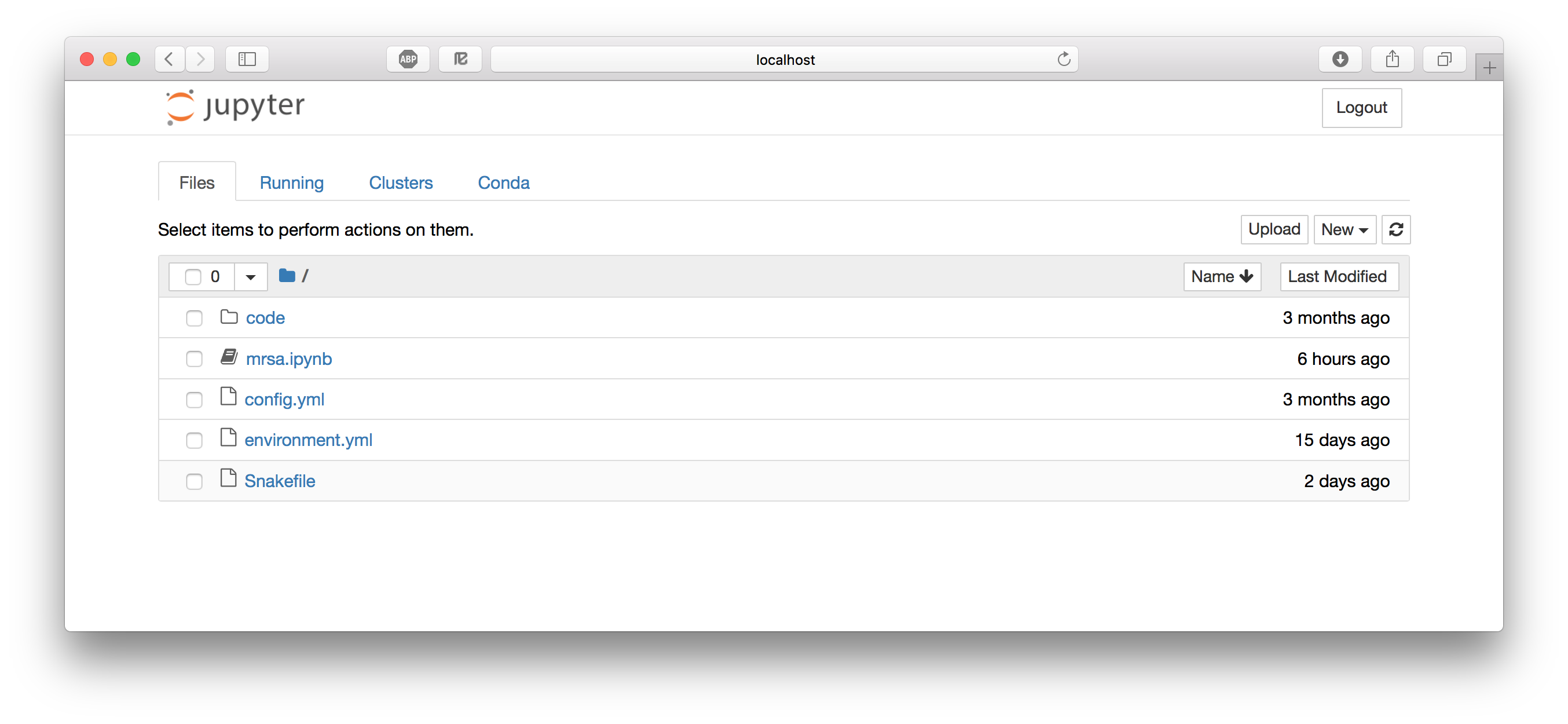
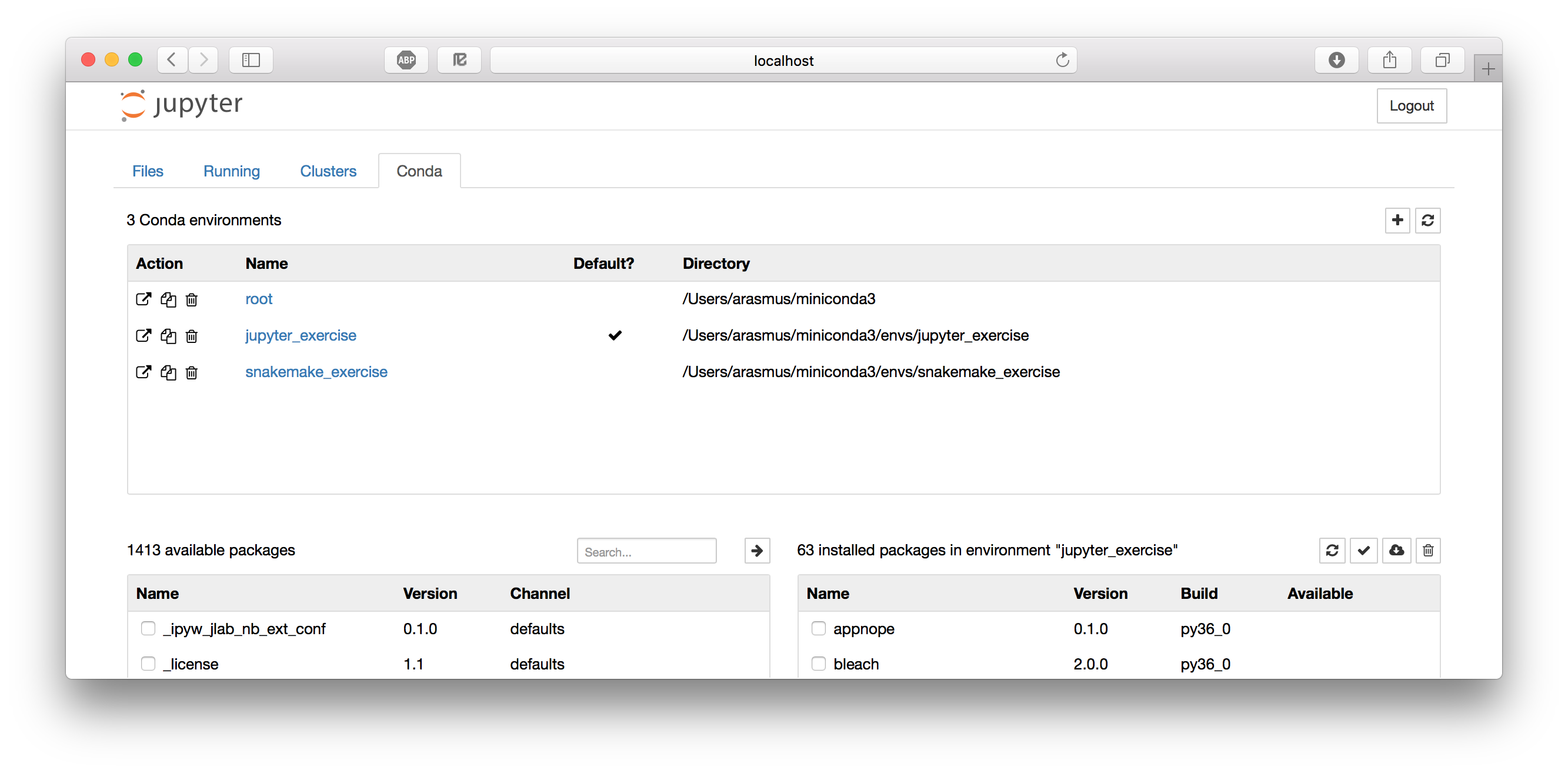
What you're looking at is the Notebook dashboard. This is where you manage your files, notebooks, and kernels. The Files tab shows the files in your directory. If you've done the other tutorials the file names should look familiar; they are the files needed for running the RNA-seq workflow in Snakemake. The Running tab keeps track of all your processes. The third tab, Clusters, is used for parallel computing and won't be discussed further in this tutorial. The Conda tab lets us control our Conda environments. Let's take a quick look at that. You can see that I'm currently in the jupyter_exercise environment.
Let's start by creating an empty notebook by selecting the Files tab and clicking New > Notebook > Python [conda env:jupyter_exercise]. This will open up a new tab or window looking like this:
![]()
Tip
If you want to start Jupyter Notebooks on a cluster that you SSH to you have to do some port forwarding:
ssh me@rackham.uppmax.uu.se -L8888:localhost:8888
jupyter notebook --ip 0.0.0.0
The very basics
Jupyter notebooks are made up out of cells, and you are currently standing in the first cell in your notebook. The fact that it's green indicates that it's in "edit mode", so you can write stuff in it. Cells in Jupyter notebooks can be of two types: markdown or code.
- Markdown - These cells contain static material such as captions, text, lists, images and so on. You express this using Markdown, which is a lightweight markup language. Markdown documents can then be converted to other formats for viewing (the document you're reading now is written in Markdown and then converted to HTML). The format is discussed a little more in detail in the R Markdown tutorial. Jupyter Notebook uses a dialect of Markdown called Github Flavored Markdown, which is described here.
- Code - These are the cells that actually do something, just as code chunks do in R Markdown. You can write code in dozens of languages and all do all kinds of clever tricks. You then run the code cell and any output the code generates, such as text or figures, will be displayed beneath the cell. We will get back to this in much more detail, but for now it's enough to understand that code cells are for executing code that is interpreted by a kernel (in this case the Python version in your Conda environment).
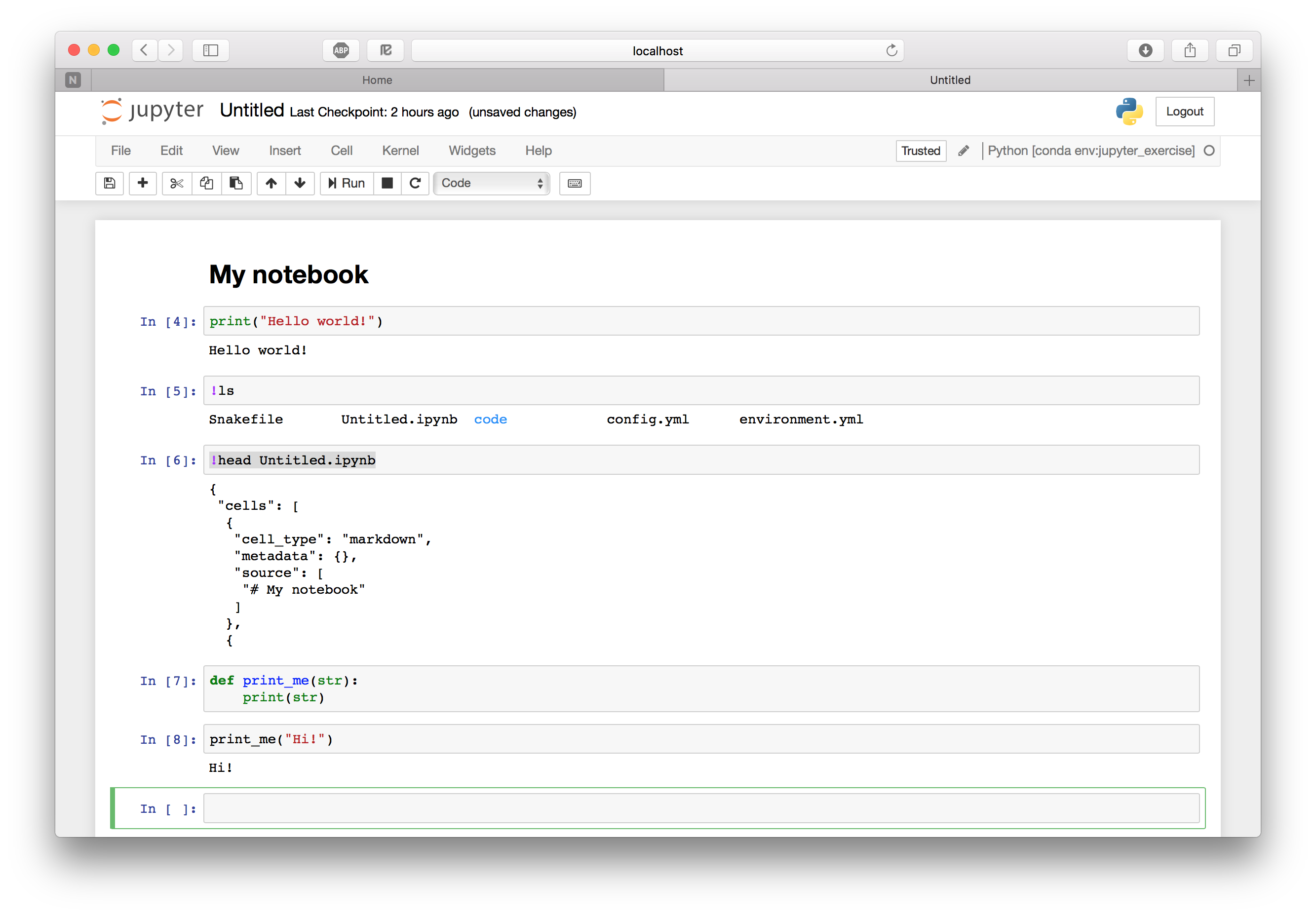
Let's use our first cell to create a header. Change the format from Code to Markdown in the drop-down list above the cell. Double click on the cell to enter editing mode (green frame) and input "# My notebook" ("#" is used in Markdown for header 1). Run the cell with Shift-Enter. Tada!
Before we continue, here are some shortcuts that can be useful. Note that they are only applicable when in command mode (blue frames). Most of them are also available from the menus.
- Enter: enter Edit mode
- Esc: enter Command mode
- Ctrl+Enter: run the cell
- Shift+Enter: run the cell and select the cell below
- Alt+Enter: run the cell and insert a new cell below
- Ctrl+S: save the notebook
- Tab: for code completion or indentation
- M/Y: toggle between Markdown and Code cells
- D-D: delete a cell
- A/B: insert cells above/below current cell
- X/C/V: cut/copy/paste cells
Now let's write some code! Since we chose a Python kernel, Python would be the native language to run in a cell. Enter this code in the second cell and run it:
print("Hello world!")
Note how the output is displayed below the cell. This interactive way of working is one of the things that sets Jupyter Notebook apart from RStudio and R Markdown. R Markdown is typically rendered top-to-bottom in one run, while you work in a Jupyter notebook in a different way. This has partly changed with newer versions of RStudio, but it's probably still how most people use the two tools. Another indication of this is that there is no (good) way to hide the code cells if you want to render your Jupyter notebook to a cleaner looking report (for a publication for example).
What is a Jupyter notebook? Let's look a little at the notebook we're currently working in. Jupyter Notebook saves it every minute or so, so you will already have it available. We can be a little meta and do this from within the notebook itself. We do it by running some shell commands in the third code cell instead of Python code. This very handy functionality is possible by prepending the command with !. Try !ls to list the files in the current directory.
Aha, we have a new file called Untitled.ipynb! This is our notebook. Look at the first ten lines of the file by using !head Untitled.ipynb. Seems like it's just a plain old JSON file. Since it's a text file it's suitable for version control with for example Git. It turns out that Github and Jupyter notebooks are the best of friends, as we will see more of later. This switching between languages and whatever-works mentality is very prominent within the Jupyter notebook community.
Variables defined in cells become variables in the global namespace. You can therefore share information between cells. Try to define a function or variable in one cell and use it in the next. For example:
def print_me(str):
  print(str)
and
print_me("Hi!")
Your notebook should now look something like this.
The focus here is not on how to write Markdown or Python; you can make really pretty notebooks with Markdown and you can code whatever you want with Python. Rather, we will focus on the Jupyter Notebook features that allow you to do a little more than that.
Quick recap
In this section we've learned:
- That a Jupyter notebook consists of a series of cells, and that they can be either markdown or code cells.
- That we execute the code in a code cell with the kernel that we chose when opening the notebook.
- We can run shell commands by prepending them with
!. - A Jupyter notebook is simply a text file in JSON format.
Magics
Magics constitute a simple command language that significantly extends the power of Jupyter notebooks. There are two types of magics:
- Line magics - Commands that are prepended by "%", and whose arguments only extend to the end of the line.
- Cell magics - Commands that start with
%%and then applies to the whole cell. Must be written on the first line of a cell.
Now list all available magics with %lsmagic (which itself is a magic). You add a question mark to a magic to show the help (e.g. %lsmagic?). Some of them act as shortcuts for commonly used shell commands (%ls, %cp, %cat, ..). Others are useful for debugging and optimizing your code (%timeit, %debug, %prun, ..).
A very useful magic, in particular when using shell commands a lot in your work, is %%capture. This will capture the stdout/stderr of any code cell and store them in a Python object. Run %%capture? to display the help and try to understand how it works. Try it out with either some Python code, other magics or shell commands.
Click to see one example
%%capture output
%%bash
echo "Print to stdout"
echo "Print to stderr" >&2
and in another cell
print("stdout:" + output.stdout)
print("stderr:" + output.stderr)
The %%script magic is used for specifying a program (bash, perl, ruby, ..) with which to run the code (similar to a shebang). For some languages it's possible to use these shortcuts:
%%ruby%%perl%%bash%%html%%latex%%R(here you have to first install the rpy2 extension, for example with Conda, and then load with%load_ext rpy2.ipython)
Try this out if you know any of the languages above. Otherwise you can always try to print the quadratic formula with LaTeX!
\begin{array}{*{20}c} {x = \frac{{ - b \pm \sqrt {b^2 - 4ac} }}{{2a}}} & {{\rm{when}}} & {ax^2 + bx + c = 0} \\ \end{array}
Python's favorite library for plotting, matplotlib, has its own magic as well: %matplotlib. Try out the code below, and you should hopefully get a pretty sine wave.
%matplotlib inline
import numpy as np
import matplotlib.pyplot as plt
x = np.linspace(0,3*np.pi,100)
y = np.sin(x)
fig = plt.figure()
ax = fig.add_subplot(111)
line, = plt.plot(x, y, 'r-')
fig.canvas.draw()
Tip
You can capture the output of some magics directly like this:
my_dir = %pwd
print(my_dir)
Widgets and interactive plotting
Since we're typically running our notebooks in a web browser, they are quite well suited for also including more interactive elements. A typical use case could be that you want to communicate some results to a collaborator or to a wider audience, and that you would like them to be able to affect how the results are displayed. It could, for example, be to select which gene to plot for, or to see how some parameter value affects a clustering. Jupyter notebooks has great support for this in the form of widgets.
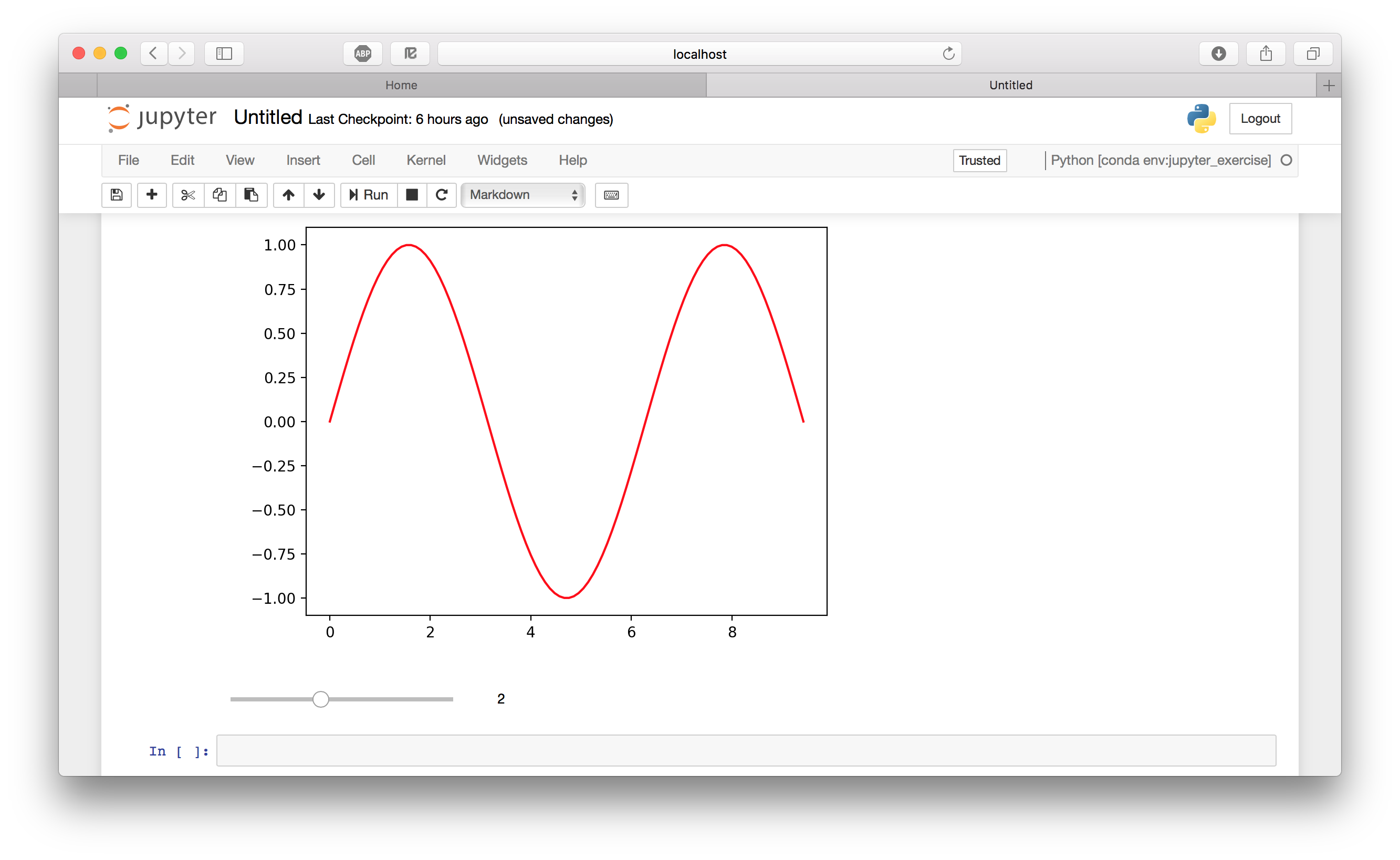
Widgets are eventful Python objects that have a representation in the browser, often as a control like a slider, textbox, etc. Let's try to add a slider that allows us to change the frequency of the sine curve we plotted previously.
%matplotlib notebook
# To use the widget framework, we need to import ipywidgets
import ipywidgets as widgets
import numpy as np
import matplotlib.pyplot as plt

# Plot default curve
x = np.linspace(0,3*np.pi,100)
y = np.sin(x)
fig = plt.figure()
ax = fig.add_subplot(111)
line, = plt.plot(x, y, 'r-')
fig.canvas.draw()

# Create and show the slider
slider = widgets.IntSlider(1, min = 0, max = 5)
display(slider)

# Define a function for modifying the line when the slider's value changes
def on_value_change(val):
    y = np.sin(x*val['new'])
    line.set_ydata(y)
    fig.canvas.draw_idle()

# Monitor for change, and send the new value to the function above on changes.
slider.observe(on_value_change, names='value')
Attention
If you have problems getting these plots to display properly, first try with restarting the kernel (under the Kernel menu). Note that this will clear any variables you have loaded.
This is how it should look if everything works. You can set the frequency of the sine curve by moving the slider.
There are lots of widgets and they all work pretty much in the same way; you listen for some event to happen and if it does you pass the new state to some function. Here is a list of all available widgets together with documentation and examples.
IPython widgets, like we used here, is the most vanilla way of getting interactive graphs in Jupyter notebooks. Some other alternatives are:
- Plotly - is actually an API to a web service that renders your graph and returns it for display in your Jupyter notebook. Generates very visually appealing graphs, but from a reproducibility perspective it's maybe not a good idea to be so reliant on a third party.
- Bokeh - is another popular tool for interactive graphs. Most plotting packages for Python are built on top of matplotlib, but Bokeh has its own library. This can give a steeper learning curve if you're used to the standard packages.
- mpld3 - tries to integrate matplotlib with Javascript and the D3js package. It doesn't scale well for very large datasets, but it's easy to use and works quite seamlessly.
Everyone likes pretty plots, so let's try one more example before we move on! This is with mpld3 and shows four subplots with shared axes. Hover over the figure and click the magnifying glass in the lower left corner. If you zoom in on a region in one plot, the others will adjust automatically. Note how seamlessly mpld3 integrates with normal matplotlib code.
%matplotlib inline
import matplotlib.pyplot as plt
import numpy as np
import mpld3

# Plot using mpld3
mpld3.enable_notebook()

# Normal matplotlib stuff
fig, ax = plt.subplots(2, 2, figsize=(8, 6),sharex='col', sharey='row')
fig.subplots_adjust(hspace=0.3)

np.random.seed(0)

for axi in ax.flat:
    color = np.random.random(3)
    axi.plot(np.random.random(30), lw=2, c=color)
    axi.set_title("RGB = ({0:.2f}, {1:.2f}, {2:.2f})".format(*color),
                  size=14)
    axi.grid(color='lightgray', alpha=0.7)
Quick recap
In the two previous sections we've learned:
- How magics can be used to extend the power of Jupyter notebooks, and the difference between line magics and cell magics.
- How to switch between different languages by using magics.
- How to use widgets and the mpld3 library for interactive plotting.
Running the MRSA workflow in a Jupyter notebook
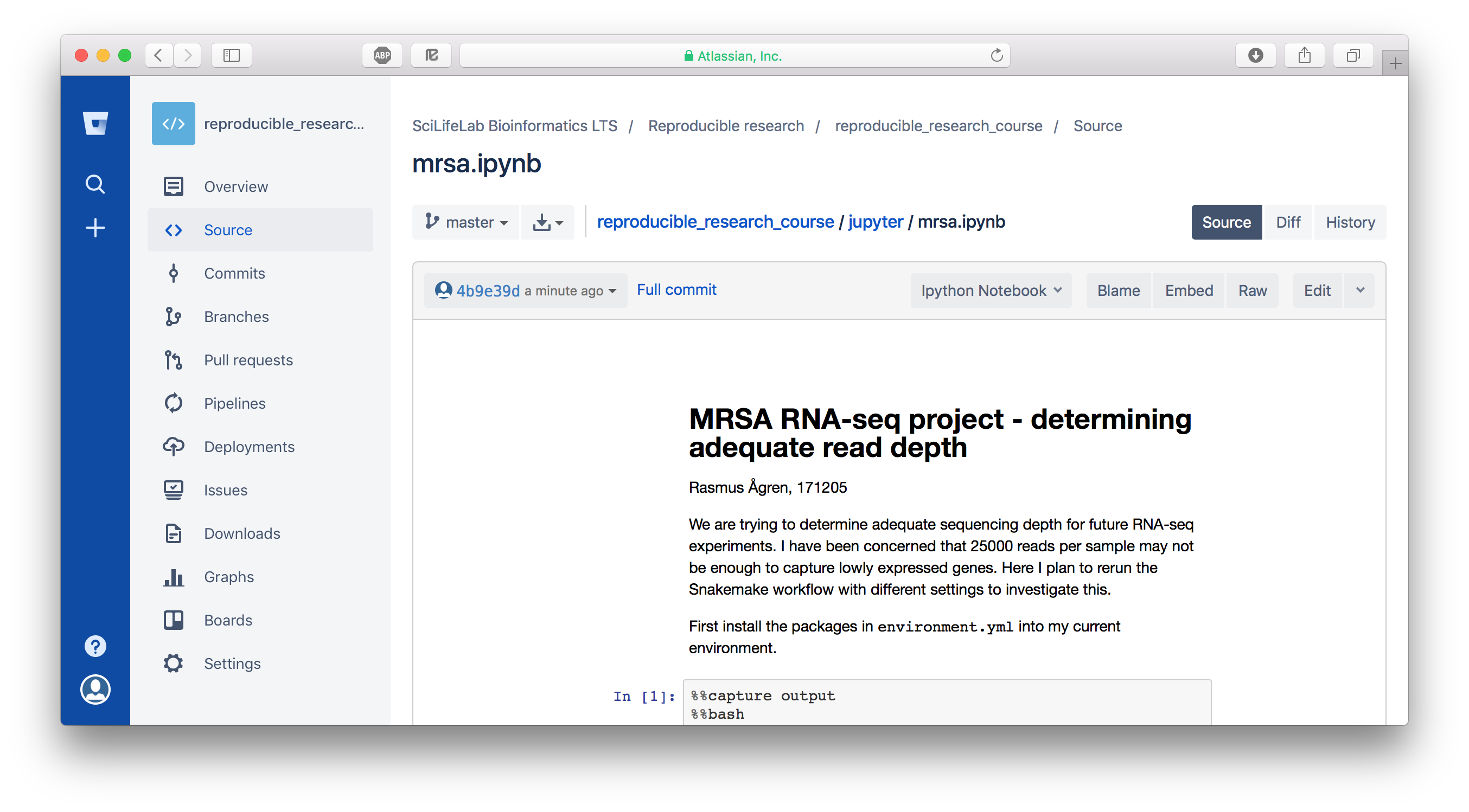
As you might remember from the intro, we are attempting to understand how lytic bacteriophages can be used as a future therapy for the multiresistant bacteria MRSA (methicillin-resistant Staphylococcus aureus). We have already defined the project environment in the Conda tutorial and set up the workflow in the Snakemake tutorial. Here we will run the workflow in a Jupyter notebook as an example of how you can document your day-to-day work as a dry lab scientist. If you look in your current directory there should be a notebook called mrsa.ipynb. Now open the notebook with File > Open.
The purpose of the notebook is to try out different settings for the max_reads parameter in our Snakemake workflow. Go through each of the cells and try to understand how they work. Now test to rerun the analysis cell by cell.
Attention
If you do something that takes a long time, such as installing the Conda environment, you have to wait for the cell to finish before trying to run the next. Running cells have asterisks to the left of them, i.e. In [*].
Sharing your work
The files you're working with come from a Bitbucket repo. Both Bitbucket and Github can render Jupyter notebooks as well as other types of Markdown documents (you need to install an extension called "Bitbucket Notebook Viewer" on Bitbucket though). Now go to our Bitbucket repo at https://bitbucket.org/scilifelab-lts/reproducible_research_course/ and navigate to jupyter/mrsa.ipynb. Change the viewer from "Default File Viewer" to "IPython Notebook".
Attention
If your Bitbucket view looks very different from the image above and you can't change the viewer, it could be that you have activated Bitbucket's "New source browser experience". It's in beta and lacks a lot of features, so you may want to disable it. If so, first click your avatar in the lower left corner, then Bitbucket Settings > Labs > New source browser experience.
As you can imagine, having this very effortless way of sharing results can greatly increase the visibility of your work. You work as normal on your project, and push regularly to the repository as you would anyways, and the output is automatically available for anyone to see. Or for a select few if you're not ready to share your findings with the world quite yet.
Say your notebook isn't on Github/Bitbucket (or you haven't activated the extension to view notebooks). All hope isn't lost there. Jupyter.org provides a neat functionality called nbviewer, where you can past an URL to any notebook and they will render it for you. Go to https://nbviewer.jupyter.org and try this out with our notebook.
https://bitbucket.org/scilifelab-lts/reproducible_research_course/raw/0f6014218b65a2bb1fdf77481995083f19bc18fa/jupyter/mrsa.ipynb
If you find all this repo stuff a little unsettling and would rather just get an old fashioned PDF to attach in an email like normal people, this is also possible. "File > Download as" lets you export your notebook to many formats, including HTML and PDF.
So far we've only shared static representations of notebooks. A strong trend at the moment is to run your notebooks in the cloud, so that the person you want to share with could actually execute and modify your code. This is a great way of increasing visibility and letting collaborators or readers get more hands-on with your data and analyses. From a reproducibility perspective, there are both advantages and drawbacks. On the plus side is that running your work remotely forces you to be strict when it comes to defining the environment it uses (probably in the form of a Conda environment or Docker image). On the negative side is that you become reliant on a third-party service that might change input formats, go out of business, or change payment model.
Here we will try out a service called Binder, which lets you run and share Jupyter Notebooks in Git repositories for free. Unfortunately it only supports GitHub, and all these tutorials live in a Bitbucket repo. We will therefore use a Github repo that we've set up to serve as a project template. The repo is available at https://github.com/NBISweden/project_template. It contains the directory structure that we've been using in these tutorials and README.md files that describe the intended contents of each directory. It also contains a minimal Conda environment, Snakemake workflow, and a Docker image to package the whole thing. Don't worry if you don't know what a Docker image is, it will be explained in the Docker tutorial.
Starting the notebook is really easy, just go to https://mybinder.org and paste the link to the GitHub repo. Note the link that you can use to share your notebook. Then press "launch".
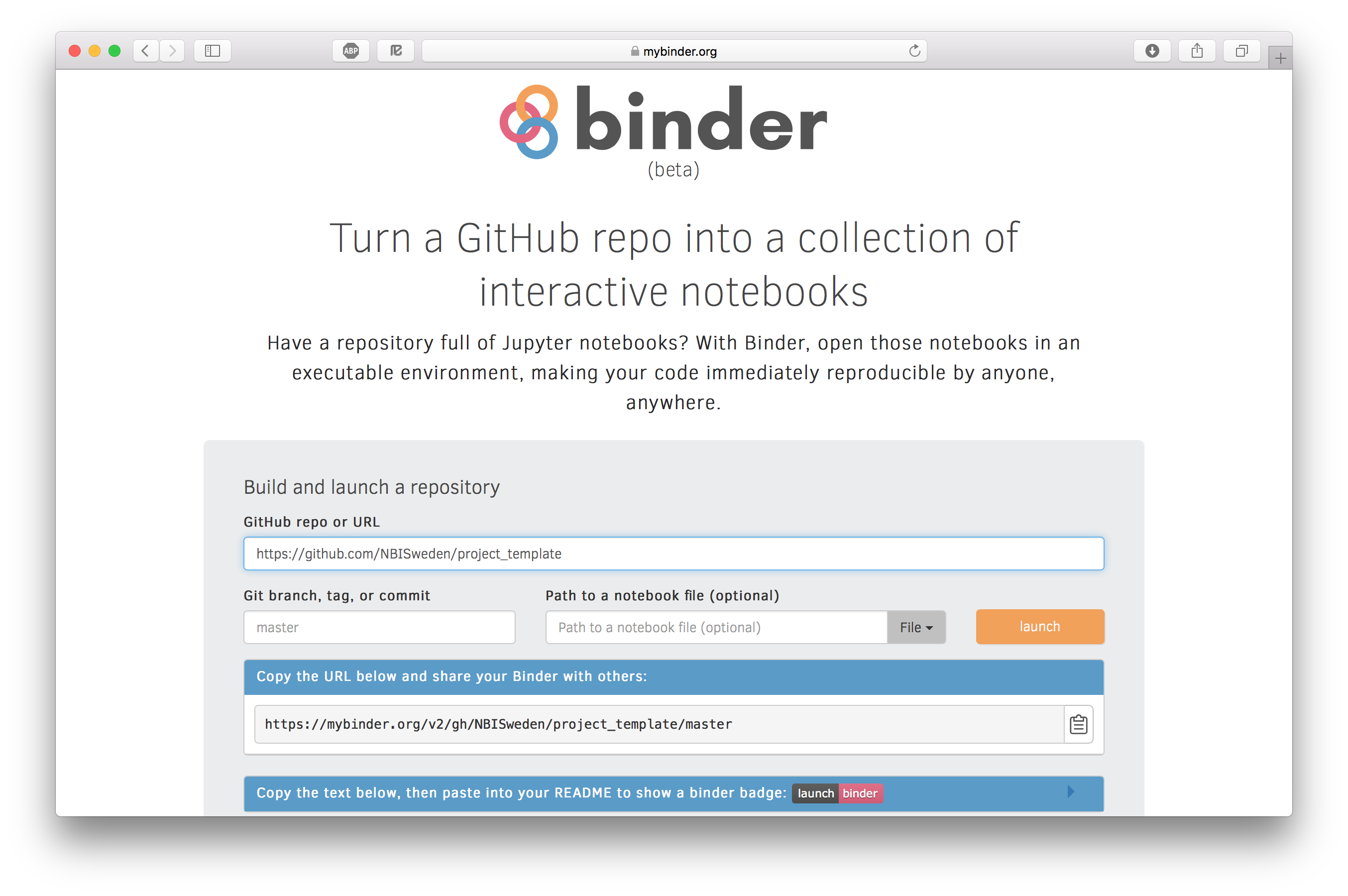
What will happen now it that:
- Binder detects that you have a file called
Dockerfilein the root of the repo. This file contains instructions for how to build the environment your notebook should run in (again, all of this is explained in the Docker tutorial). Binder then builds a Docker image based on the file. This might take a minute or two. You can follow the progress in the build log. - Binder then launches the Jupyter Notebook server in the Docker image..
- ..and opens a browser tab with it for you.
The repo contains a notebook template in the notebooks directory. Open it and execute the first code cell. Tada! While a little underwhelming to the untrained eye, this is actually kind of cool. We now have a way to run our analyses in the cloud and in an environment that we define ourselves. All that's needed for someone to replicate your analyses is that you share a link with them. Note that notebooks on Binder are read-only; its purpose is for trying out and showing existing notebooks rather than making new ones.
A note on transparency
Resources like Github/Bitbucket and Jupyter Notebooks have changed the way we do scientific research by encouraging visibility, social interaction and transparency. It was not long ago that the analysis scripts and workflows in a lab were well-guarded secrets that we only most reluctantly shared with others. That assuming that it was even possible. In most cases, the only postdoc who knew how to get it to work had left for a new position in industry, or no one could remember the password to the file server. If you're a PhD student, we encourage you to embrace this new development wholeheartedly, for it will make your research better and make you into a better scientist. And you will have more fun.